Background

I have a goal of stacking Jenga blocks. But before the robot arm can do anything fancy, I need to stop being scared of images.

Short Goal

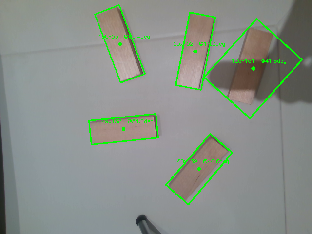
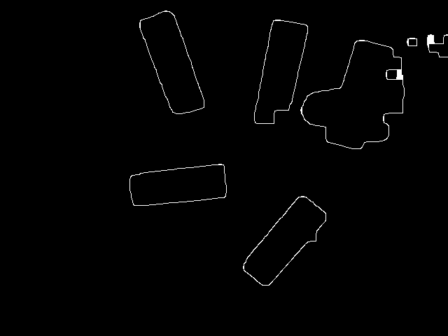
So I started with this static photo of Jenga blocks from my desktop camera. The small mission: draw accurate rotated boxes, center dots, and labels around the blocks by the end of this post.

Original RealSense camera image with five Jenga blocks on a table
The starting photo: five blocks, 640 x 480 pixels, shot with an Intel RealSense D435. The lighting is not perfect, the shadow is dramatic, and OpenCV is about to judge me.

After some trial, error, and mild emotional damage, this became the first usable output:

Detected Jenga blocks with green rotated boxes, center dots, and angle labels
Green boxes, center dots, sizes, and angles. The blocks are mostly found. The shadow on the right is still trying to become famous.

And the stupidity begins…

OpenCV 1

1
2
import cv2 as lv
import numpy as np

Typically, people import cv2 as cv, but why not make it un poco luxurious? lv sounds richer to me. HAHAH!

Do Not Be Afraid by OpenClaw

OpenClaw once said, “yeah, I got you.”

📄 opencv.pdf - OpenClaw's "yeah, I got you" notes

Reference Sample

Check this only if you’re out of time. For me, I find it useless for personal growth and critical thinking.

Show/hide sample Python code
1
2
3
4
5
6
7
8
9
10
11
12
13
14
15
16
17
18
19
20
21
22
23
24
25
26
27
28
29
30
31
32
33
34
35
36
37
38
39
40
41
42
43
44
45
46
47
48
49
50
51
52
53
54
55
56
57
58
59
60
61
62
63
64
65
66
67
68
69
70
71
72
73
74
75
76
77
import cv2
import numpy as np

# === LOAD IMAGE ===
img = cv2.imread('cv.png')
h, w = img.shape[:2]
print(f"Image: {w}x{h}")

# === STEP 1: HSV COLOR SEGMENTATION ===
# Wooden blocks: warm hue (H < 20), moderate-to-high saturation (S > 25)
# Saturation is the key — table is desaturated, blocks have color
hsv = cv2.cvtColor(img, cv2.COLOR_BGR2HSV)
lower = np.array([0, 25, 0]) # H, S, V
upper = np.array([20, 255, 255])
mask = cv2.inRange(hsv, lower, upper)

# === STEP 2: MORPHOLOGY — clean up mask ===
kernel = cv2.getStructuringElement(cv2.MORPH_RECT, (5, 5))
mask = cv2.morphologyEx(mask, cv2.MORPH_CLOSE, kernel, iterations=2)
mask = cv2.morphologyEx(mask, cv2.MORPH_OPEN, kernel, iterations=1)

# === STEP 3: GAUSSIAN BLUR before Canny ===
# Smooths noise and wood grain → cleaner edge detection
blurred = cv2.GaussianBlur(mask, (5, 5), 0)

# === STEP 4: CANNY EDGE DETECTION ===
edges = cv2.Canny(blurred, 50, 150)
edges = cv2.morphologyEx(edges, cv2.MORPH_CLOSE, kernel, iterations=2)

# === STEP 5: FIND CONTOURS ===
contours, _ = cv2.findContours(edges, cv2.RETR_EXTERNAL, cv2.CHAIN_APPROX_SIMPLE)

result = img.copy()
blocks = []

for cnt in contours:
area = cv2.contourArea(cnt)
if area < 1000:
continue # noise threshold

# === STEP 6: ROTATED BOUNDING BOX ===
# minAreaRect returns: (center=(cx,cy), size=(w,h), angle=degrees)
# angle is relative to the horizontal axis
rect = cv2.minAreaRect(cnt)
box = cv2.boxPoints(rect).astype(int)
rw, rh = rect[1]
aspect = rw / float(rh) if rh > 0 else 0

# Filter by size/aspect ratio
if 0.2 < aspect < 6.0 and area > 2000:
cx, cy = int(rect[0][0]), int(rect[0][1])
blocks.append({"rect": rect, "area": area})

# Draw rotated rectangle
cv2.drawContours(result, [box], 0, (0, 255, 0), 2)
# Center dot
cv2.circle(result, (cx, cy), 4, (0, 255, 0), -1)
# Label: width x height @ angle
label = f"{rw:.0f}x{rh:.0f} @{rect[2]:.1f}deg"
cv2.putText(result, label, (cx - 45, cy - 12),
cv2.FONT_HERSHEY_SIMPLEX, 0.35, (0, 255, 0), 1)

print(f"\nPipeline: HSV → GaussianBlur(5x5) → Canny(50,150) → minAreaRect")
print(f"Found {len(blocks)} blocks:")
for i, b in enumerate(blocks):
r = b["rect"]
print(f" Block {i+1}: {r[1][0]:.0f}x{r[1][1]:.0f} "
f"at ({r[0][0]:.0f},{r[0][1]:.0f}), "
f"angle={r[2]:.1f}deg, area={b['area']:.0f}")

# === SAVE ===
# cv2.imwrite('cv_detected.png', result)
# cv2.imwrite('cv_edges.png', edges)

cv2.imshow('result', result)
cv2.waitKey(0) # wait for a key press
cv2.destroyAllWindows() # close the window

Basic

If you know this, simply skip :)

1
2
3
4
5
6
7
8
9
10
11
12
13
import numpy as np

a = np.array([1.1, 2.0, 3.6, 4.8, 5.9])

b = np.array([
[1, 2, 3],
[1, 2, 3],
[1, 2, 3],
[1, 2, 3],
])

print(a.shape)
print(b.shape)

Output:

1
2
(5,)
(4, 3)

Explanation:

  • shape returns a tuple.
  • Each number in the tuple tells you how many elements exist along that dimension.
  • a is one-dimensional, so its shape is (5,).
  • b has 4 rows and 3 columns, so its shape is (4, 3).

What about if we print:

1
2
print(a.dtype)
print(b.dtype)

Output:

1
2
float64
int32

It is obvious that dtype is simply short for dog Type, um, data type I mean.

Dictionaries

1
2
3
4
5
6
block2 = dict(
center_uv=(100, 200),
angle_deg=10,
score=0.7,
depth=0.3
)

Imagine this is an actual block with values appended to the dictionary.

Question:

How should I access the values in the bracket?

1
print(block2["score"])

Output:

1
0.7

OK, this sounds nice, but what if there is no key, such as shadow? An alternative method is .get():

1
print(block2.get("shadow", "No such key!"))

Output:

1
No such key!

Iterating Over a Dictionary

The default method that I first learned is:

1
2
for item in block2:
print(item, block2[item])

Output:

1
2
3
4
center_uv (100, 200)
angle_deg 10
score 0.7
depth 0.3

But there is a more elegant method by using .items() and an f-string.

1
2
for key, value in block2.items():
print(f"key: {key}, value: {value}")

Output:

1
2
3
4
key: center_uv, value: (100, 200)
key: angle_deg, value: 10
key: score, value: 0.7
key: depth, value: 0.3

.items() gives you both the key and value directly.

Lambda

Normally when you write a function:

1
2
def get_score(block):
return block['score']

With lambda, you don’t need to write a full function. I think of it as a small one-use function.

1
2
3
get_score_lambda = lambda b: b['score']

print(get_score_lambda(block2))

Output:

1
0.7

Example: Nested Dictionaries

1
2
3
4
5
6
7
8
9
10
11
12
13
14
15
16
17
18
19
20
21
22
23
24
detection_result = {
"frame_id": 12,
"timestamp": 12345415465,
"blocks": [
{
"center_uv": (120, 240),
"angle_deg": 88,
"depth": 0.67,
"score": 0.67
},
{
"center_uv": (320, 240),
"angle_deg": -22,
"depth": 0.4,
"score": 0.93
}
],
"camera_info": {
"width": 640,
"height": 480,
"fx": 615,
"fy": 615
}
}

We have two blocks in this dictionary. What should I do when I want to find the best score and the greatest depth?

1
2
3
4
5
6
7
best, deepest = (
max(detection_result["blocks"], key=lambda b: b["score"]),
max(detection_result["blocks"], key=lambda b: b["depth"])
)

print(f"best: {best}")
print(f"deepest: {deepest}")

Output:

1
2
best: {'center_uv': (320, 240), 'angle_deg': -22, 'depth': 0.4, 'score': 0.93}
deepest: {'center_uv': (120, 240), 'angle_deg': 88, 'depth': 0.67, 'score': 0.67}

Enumerate

In simple terms, enumerate() provides you with both the index and the value simultaneously.

Without enumerate():

1
2
3
4
centers = [(100, 200), (300, 150), (250, 310)]

for i in range(len(centers)):
print(i, centers[i])

With enumerate():

1
2
for i, value in enumerate(centers):
print(i, value)

OpenCV 2: From Color to Edges

OpenCV loads images in BGR order, not RGB.

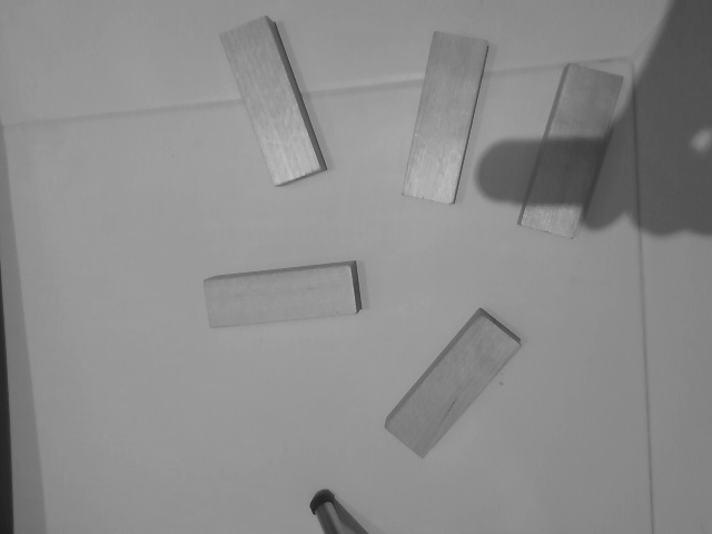
In this project, I tested multiple options such as Lab and HSV.
I realized that Saturation outperforms the others for this setup.

Set Up

1
2
3
4
5
6
7
8
9
import numpy as np
import cv2 as lv

img = lv.imread('cv.png')
if img is None:
print('No such image!')
exit(1)

print(f'Original Shape: {img.shape[1]}x{img.shape[0]}')

Explanation:

  • lv.imread('cv.png') tries to load the image.
  • If the image does not exist, img becomes None.
  • A normal program exit would be exit(0).
  • Since missing cv.png is an error, this uses exit(1).

HSV Channels

1
2
3
hsv = lv.cvtColor(img, lv.COLOR_BGR2HSV)

h_ch, s_ch, _ = lv.split(hsv)

Explanation:

  • cvtColor converts the image from BGR into HSV.
  • split separates the image into hue, saturation, and value channels.
  • _ means “I am intentionally ignoring this value.”

During this period, I was still struggling to determine if hue or saturation works better. Still, I decided to separate them during the preprocessing step.

Gaussian Blur

1
s_blur = lv.GaussianBlur(s_ch, (5, 5), 0)

Explanation:

  • One obstacle that hinders Canny from identifying edges is NOISE and rough pixel transitions.
  • Once this (5, 5) Gaussian blur is applied, each pixel becomes an average of its 5x5 neighborhood.
  • This preprocessing step is vital because it increases the efficiency and accuracy of the actual detection.
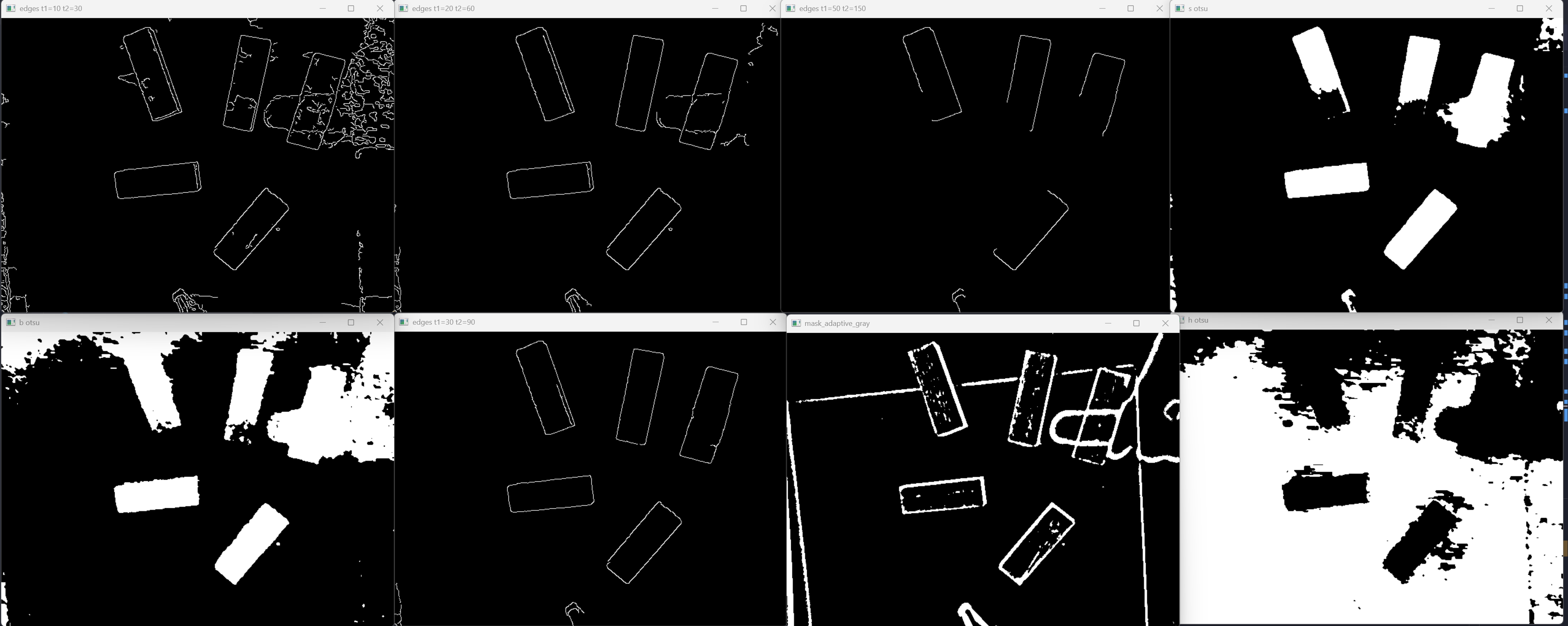
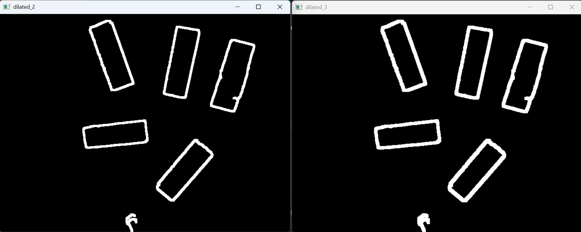
📄 gaussian_blur.pdf - because the pixels need to calm down

Visual Checkpoints

Below are the screenshots I kept while tuning the pipeline. This is the part where computer vision stops feeling like magic and starts feeling like arguing with pixels.

Grayscale version of the Jenga block test image
Grayscale version. The blocks are still visible, but the useful wood color is gone. A little too elegant, a little too useless.
Comparison grid of edge detection and thresholding experiments
A small gallery of experiments: Canny thresholds, Otsu masks, and adaptive thresholding. Some found the blocks. Some found the meaning of chaos.
Side-by-side dilation results showing thick white outlines around the blocks
Dilation test. Thicker outlines make contours easier to grab, but if I push it too far, the noise also gets promoted.
Final edge map with white outlines of the blocks on a black background
Final-ish edge map. The five blocks are there, mostly behaving. The right-side shadow is still applying for block citizenship.

Live Preview and Short Demo

Canva preview. It stays 16:9 because this one is a slide-like canvas, not a phone video pretending to be a rectangle.

YouTube Short. Strict 9:16. Vertical video deserves to remain vertical.