When a Pig Started to Learn OpenCV... and Ended Up Moving a Robot Arm
Background
I have a goal of stacking Jenga blocks with a robot arm. Not in simulation — with
real hardware that can actually knock things over. The setup ended up being an Intel
RealSense depth camera bolted to the wrist of a UFactory xArm (an eye-in-hand
rig), OpenCV finding the best block in the frame, and the arm picking it up and
placing it on a growing stack.
But before any of that fancy motion, I needed to stop being scared of images.
Short Goal
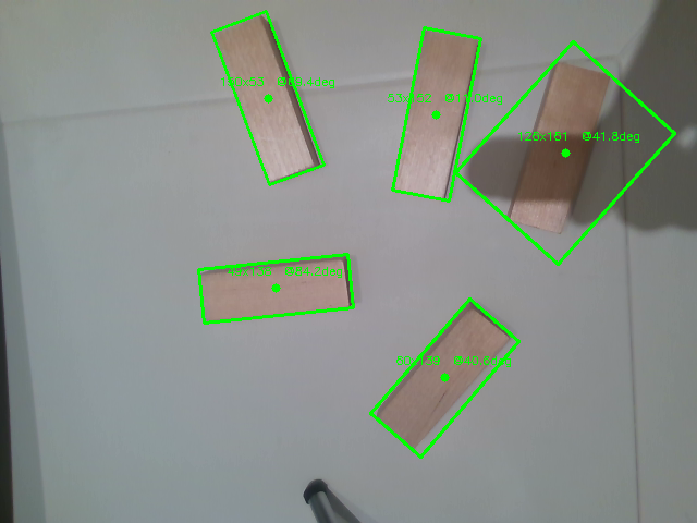
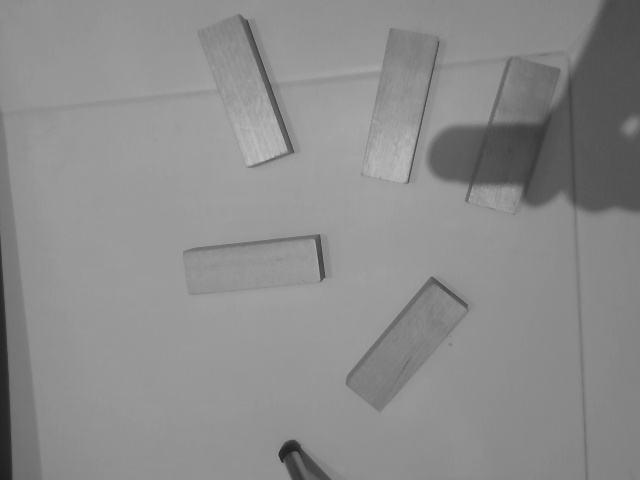
So I started with this static photo of Jenga blocks from my desktop camera. The small
mission: draw accurate rotated boxes, center dots, and labels around the blocks by the
end of this post — and then, much later, turn those boxes into 3D points the robot can
actually reach.

After some trial, error, and mild emotional damage, this became the first usable output:
This post follows the whole road: from “what even is a pixel” to a real arm picking a
block off the table. Each section is one skill I had to learn, plus how it bolts onto
the one before it.
And the stupidity begins…
OpenCV 1
1 | import cv2 as lv |
Typically, people import cv2 as cv, but why not make it un poco luxurious? lv sounds richer to me. HAHAH!
Everything below uses
lvfor OpenCV. In the actual repo it is the boringcv2, but here we stay rich.
Do Not Be Afraid by OpenClaw
OpenClaw once said, “yeah, I got you.”
Before the panic sets in, it helps to know what “computer vision” even means. Columbia’s
Prof. Shree Nayar gives the calmest possible answer:
Basic
If you know this, simply skip :)
1 | import numpy as np |
Output:
1 | (5,) |
Explanation:
shapereturns atuple.- Each number in the tuple tells you how many elements exist along that dimension.
ais one-dimensional, so its shape is(5,).bhas 4 rows and 3 columns, so its shape is(4, 3).
This matters more than it looks: an OpenCV image is a numpy array. A color frame is(480, 640, 3) — height, width, then 3 color channels. Knowing which axis is which
saves you from a lot of “why is my image sideways” moments later.
What about if we print:
1 | print(a.dtype) |
Output:
1 | float64 |
It is obvious that dtype is simply short for dog Type, um, data type I mean.
Dictionaries
1 | block2 = dict( |
Imagine this is an actual block with values appended to the dictionary. Hold onto this
shape — by the end of the post, the real detector hands back a dictionary that looks
almost exactly like this, with center_uv, angle_deg, score, and a depth.
Question:
How should I access the values in the bracket?
1 | print(block2["score"]) |
Output:
1 | 0.7 |
OK, this sounds nice, but what if there is no key, such as shadow? An alternative method is .get():
1 | print(block2.get("shadow", "No such key!")) |
Output:
1 | No such key! |
Iterating Over a Dictionary
The default method that I first learned is:
1 | for item in block2: |
Output:
1 | center_uv (100, 200) |
But there is a more elegant method by using .items() and an f-string.
1 | for key, value in block2.items(): |
Output:
1 | key: center_uv, value: (100, 200) |
.items() gives you both the key and value directly.
Lambda
Normally when you write a function:
1 | def get_score(block): |
With lambda, you don’t need to write a full function. I think of it as a small one-use function.
1 | get_score_lambda = lambda b: b['score'] |
Output:
1 | 0.7 |
This exact trick is how the detector later picks a winner: max(blocks, key=lambda b: b["score"]).
Example: Nested Dictionaries
1 | detection_result = { |
We have two blocks in this dictionary. What should I do when I want to find the best score and the greatest depth?
1 | best, deepest = ( |
Output:
1 | best: {'center_uv': (320, 240), 'angle_deg': -22, 'depth': 0.4, 'score': 0.93} |
Notice camera_info already carries fx and fy — the focal lengths. Those two
numbers are what turn a flat pixel into a real 3D point much later. Foreshadowing.
Enumerate
In simple terms, enumerate() provides you with both the index and the value simultaneously.
Without enumerate():
1 | centers = [(100, 200), (300, 150), (250, 310)] |
With enumerate():
1 | for i, value in enumerate(centers): |
OpenCV 2: From Color to Edges
OpenCV loads images in BGR order, not RGB.
In this project, I tested multiple options such as Lab and HSV.
I realized that Saturation outperforms the others for this setup — the table is
washed-out and gray, while the wooden blocks actually have color. Saturation is exactly
“how colorful is this pixel,” so it separates wood from table almost for free.
Set Up
1 | import numpy as np |
Explanation:
lv.imread('cv.png')tries to load the image.- If the image does not exist,
imgbecomesNone. - A normal program exit would be
exit(0). - Since missing
cv.pngis an error, this usesexit(1).
HSV Channels
1 | hsv = lv.cvtColor(img, lv.COLOR_BGR2HSV) |
Explanation:
cvtColorconverts the image fromBGRintoHSV.splitseparates the image into hue, saturation, and value channels._means “I am intentionally ignoring this value.”
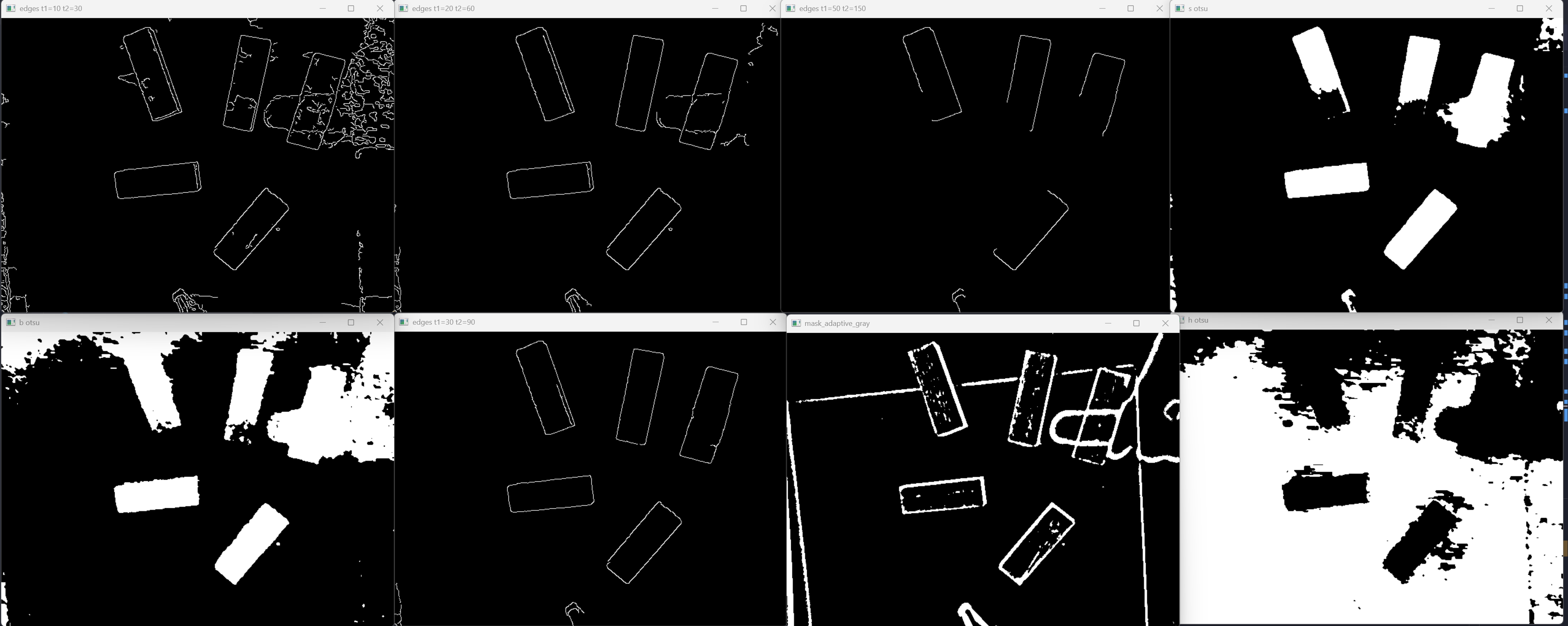
During this period, I was still struggling to determine if hue or saturation works better. Still, I decided to separate them during the preprocessing step.
So I just stared at single channels and thresholds until one of them looked like a block
and not like modern art:


Shadow Normalization
Saturation handles color, but it does nothing about uneven lighting. One side of the
table is bright, the other is in shadow, and a naive threshold either keeps the shadow
or loses the dim blocks. So before thresholding, I flatten the lighting.
The trick: take the L (lightness) channel, boost local contrast with CLAHE, then
divide the image by a heavily blurred copy of itself. The blurred copy is the slow
lighting gradient, so dividing it out leaves only the fast detail — the blocks.
1 | def shadow_normalized_luma(img): |
CLAHEis “adaptive histogram equalization” — it brightens dark patches without
blowing out the bright ones.lv.divide(..., scale=255)rescales so the result is still a normal 0–255 image.
Gaussian Blur
1 | s_blur = lv.GaussianBlur(s_ch, (5, 5), 0) |
Explanation:
- One obstacle that hinders
Cannyfrom identifying edges is NOISE and rough pixel transitions. - Once this
(5, 5)Gaussian blur is applied, each pixel becomes an average of its5x5neighborhood. - This preprocessing step is vital because it increases the efficiency and accuracy of the actual detection.
Canny and Threshold Tuning
Canny finds edges by looking for sharp brightness changes. It takes two thresholds —
a low one and a high one — and honestly the only way I understood them was to open six
windows at once and stare:
1 | edges = lv.Canny(blur, 30, 70) # (low, high) — too low = static, too high = nothing |
If you want the actual reason those two numbers exist (the “hysteresis” trick), Computerphile explains Canny better than I ever could:


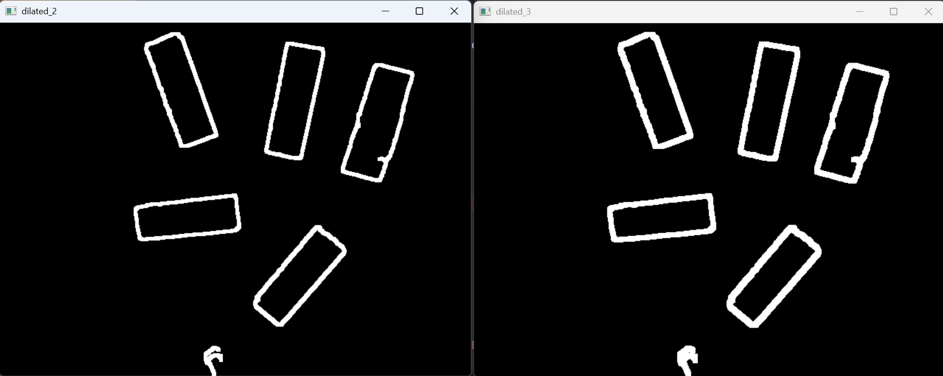
Morphology
Canny gives me thin, broken outlines. To turn them into a solid shape I need
morphology — grow the edges a little (dilate), then close the gaps
(MORPH_CLOSE):
1 | kernel = lv.getStructuringElement(lv.MORPH_RECT, (3, 3)) |
Experiment Gallery
Before I settled on the pipeline above, I threw everything at the wall. These are the
screenshots I kept while losing my mind:
Two Masks, OR’d Together
Edges alone are fragile — one shadow and the outline breaks. Color alone is fragile too —
one bright reflection and a block goes missing. So the real pipeline builds two masks
and combines them with bitwise_or, on the theory that a pixel is probably a block if
either test agrees.
Color mask — threshold the LAB b channel (blue ↔ yellow) and the HSV saturation,
each with Otsu, which picks its own threshold automatically:
1 | lab = lv.cvtColor(img, lv.COLOR_BGR2LAB) |
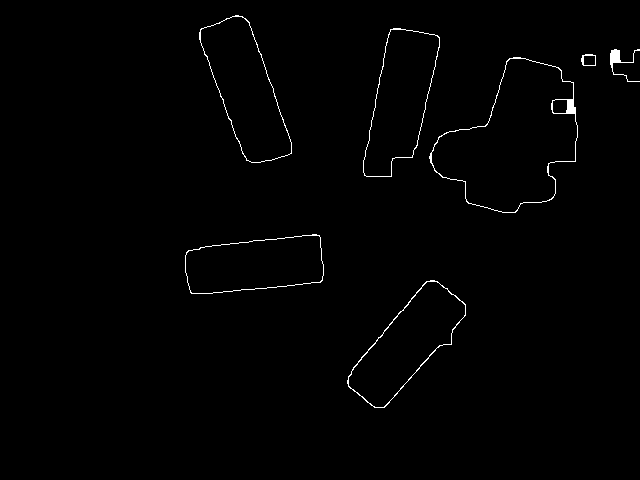
Edge-fill mask — take the closed edges from before, find the outer contours, and
fill them in so each outline becomes a solid blob. Then bitwise_or the two masks
together.

On real wooden blocks (the live rig, not the test photo) the same mask looks like this —
and notice the little marker on the top block, which I used as a sanity reference:

Watershed: Splitting Blocks That Touch
Here is a problem the test photo hides: when two blocks touch, the mask glues them into
one fat blob, and minAreaRect then draws one giant wrong box. The fix is
watershed — treat the mask like a landscape and “flood” it from the center of each
block so the seam between them becomes a wall.
1 | dist = lv.distanceTransform(mask, lv.DIST_L2, 5) # how deep inside each blob |
distanceTransformmeasures how far each white pixel is from the nearest black one —
the centers of blocks are “deepest.”connectedComponentsgives each separate center its own number, so two touching
blocks become two labels instead of one.watershedgrows those labels until they meet, drawing a boundary exactly where two
blocks touch.
The “treat the image like a landscape and flood the valleys” picture is hard to get from
words alone, so here it is animated:
Finding the Block
Now the mask is clean and split, so I can finally measure each block. For every contour:
filter by area, find the center with moments, and find the size + angle withminAreaRect.
1 | contours, _ = lv.findContours(mask, lv.RETR_EXTERNAL, lv.CHAIN_APPROX_SIMPLE) |
Scoring: which blob is actually a Jenga block?
Lots of things make rectangles. To pick the real block I give each candidate a
score — a weighted blend of four “does this look right” questions, each shaped so
that “close to the expected block” scores near 1:
1 | fill_score = min(area / (long_px * short_px), 1.0) # how filled-in is the box? |
Then I sort candidates by score and take the best — the max(..., key=lambda b: b["score"])
trick from the dictionaries section, finally paying off. Each detection comes back as a
dictionary that looks an awful lot like block2 from way back: center_uv, angle_deg,score, and friends.
The angle from minAreaRect becomes the gripper yaw after normalizing it to a sane
range, so the gripper can line up with the block:
1 | def normalize_angle(deg): |

The pipeline on real blocks
Stepping through the actual debug images the program writes on every grab — raw frame,
binary mask, final pick:


Adding Depth: From Pixels to 3D
A green box is nice, but the robot lives in millimeters, not pixels. The RealSense gives
me a depth image aligned to the color image, so every pixel also has a distance.
1 | align = rs.align(rs.stream.color) # make depth line up with color |
Raw depth is noisy and full of holes, so for the block center I take a median of the
valid depths in a small patch (and fall back to the median inside the contour if the
center pixel is a dropout). A median shrugs off the zeros that wreck an average.
Then the actual magic — back-projection — turns a pixel (u, v) plus its depth into
a real camera-frame point in meters, using the camera’s focal lengths and optical center:
1 | def pixel_to_3d(u, v, depth_m, fx, fy, cx, cy): |
Those fx, fy are the same focal lengths hiding in the camera_info dictionary from
the Dictionaries section. Everything connects.
Where do fx, fy, cx, cy even come from? They are the linear camera model. Columbia’s
First Principles of Computer Vision lays it out cleanly — this is the math my four
mystery numbers are quietly obeying:
fx, fy, cx, cy actually come from, and why back-projection is just running it backwards.
To actually see depth, you colorize it. Near is bright, far is dark — here is a fist
held in front of the camera, which is exactly the kind of thing that breaks naive color
masks but reads beautifully in depth:

Put it together and a single detection now carries a real 3D position, a yaw, and a
confidence score:

z=0.285m, yaw — the block is no longer a picture, it is a place in space the arm can reach.
Going Live
A static photo is a comfortable lie. The real rig runs on a live stream so I can move
the camera around and watch detections update in real time. Instead of capturing one
frame, I keep the RealSense pipeline open and loop:
1 | while True: |
The overlay shows the live score, depth, yaw, an FPS counter, and how many blocks are in
the stack so far. Press g and the arm grabs whatever is currently highlighted.


A Detour: Pointing It at My Face
Once the pipeline worked, I obviously pointed it at things that are not Jenga blocks,
because that is the law. The same HSV/skin logic happily detects a face, and depth
happily measures a hand. Useless for stacking, excellent for morale.


From Camera to Robot
The detector gives me a point in the camera’s frame. The robot thinks in the
base frame. Because the camera rides on the wrist (eye-in-hand), there is no single
fixed transform — the camera moves with every joint. So at the moment of capture I read
the live wrist pose and chain two transforms:
1 | point_base = T_base_from_tcp_current @ T_tcp_from_camera @ point_camera |
T_tcp_from_camerais the measured mount: where the camera sits relative to the
tool, in millimeters and degrees. Measure it once, mark itverified, or the script
refuses to move (a safety I was grateful for more than once).T_base_from_tcp_currentis the live wrist pose, read the instant the frame is taken.
If the @ (matrix multiply) and the idea of a “rotation matrix” feel like hand-waving,
this is the one video that made it click for me — a matrix is just a transformation of
space, and a rotation is one of them:
The gripper yaw gets its own little equation, combining the wrist’s current yaw, the
block’s vision yaw, and a 90° offset for grabbing the long side:
1 | pick_yaw = capture_yaw - vision_yaw + yaw_offset + wrist_grasp_offset # +90 for long side |
Before anything moves, every target is checked against a safe-range box (a min/max
XYZ volume in the config). Outside the box → the move is refused. Then the arm runs a
plain, boring, beautiful 9-step pick-and-place: open gripper, rise to a safe height, go
above the block, descend, close, lift, go above the place spot, descend, release.
This is the panel I used to jog the arm and watch its live pose while tuning all of the
above:

Stacking
One pick is a party trick; a tower is the goal. The stacking math is deliberately simple:
two blocks per layer, side by side, offset by the block width (25 mm). Each new layer is
raised by the block height (15 mm) and rotated 90° from the one below — the classic Jenga
weave. Between every move the arm lifts to a travel-height clearance so it never plows
through the stack it just built.
The block dimensions, the place position, the safe box, and the gripper open/close values
all live in config2.json, so re-tuning the tower never touches the code.
Reading the Debug Images
A robot that grabs the wrong block is useless if I can’t see why. So every time I pressg, the program dumps four images into grab_debug/ — plus a numbered copy each cycle
(detection_001.png, detection_002.png, …) so the whole stacking run replays frame by
frame afterward. These four are the entire debugging toolkit:
color.png— the raw camera frame. What the camera actually saw: lighting, glare,
and every block on the table.depth_raw.png— the 16-bit depth frame. Whether there is real depth where the
block is. Holes here mean trouble.mask.png— the binary segmentation. Did the pipeline find clean block shapes, or
glue two touching blocks into one fat blob?detection.png— the final labeled pick. Which block won, and its score, depth, and
yaw.
Debugging is just reading them in order. Robot missed entirely? The mask shows
whether two blocks fused (a watershed problem) or a block vanished (a threshold problem).
Picked a strange block? The detection label shows the winning score — usually something
non-block scored too high. Lunged to the wrong height? The depth_raw had a hole right at
the center, so the median depth fell back to something silly. (You already met this set as
the color → mask → detection row up in Finding the Block.)
The depth frame, made visible
depth_raw.png looks pure black to the eye, because its values are tiny raw units — in
this frame, 0 to 418 out of a 16-bit range. Colorize it and the scene appears: the blocks
sit closer to the wrist camera (blue) than the table (red), which is exactly the signal
the 3D back-projection needs. The black freckles are depth dropouts the median has to
survive.

One run, frame by frame
The numbered detection_* images are the receipts for a full stacking session. Early on
the table is crowded; the detector keeps locking onto the highest-scoring block, the arm
clears it, and a couple dozen grabs later the table is nearly empty:


Live Preview and Short Demo
Canva preview. It stays 16:9 because this one is a slide-like canvas, not a phone video pretending to be a rectangle.
YouTube Short. Strict 9:16. Vertical video deserves to remain vertical.
Skills I Picked Up
A quick honest inventory of what this little pig actually learned, start to finish:
- OpenCV — color spaces (BGR/HSV/LAB), CLAHE shadow normalization, Otsu thresholds,
Canny + morphology, watershed to split touching blocks, contours,moments,minAreaRect, and a weighted scoring function to choose the real block. - Depth camera — aligning depth to color, reading intrinsics and depth scale, robust
median depth, and back-projecting a pixel into a real 3D point. - Calibration — the eye-in-hand transform chain, and why a wrist-mounted camera can’t
use one fixed matrix. - Robot motion — talking to an xArm, gripper control, safe-range checks, a 9-step
pick-and-place, and the stacking math that turns single grabs into a tower.
The pig is no longer scared of images. The pig now has a robot arm. This was probably a
mistake.